Bayesians Commit the Gambler's Fallacy

And they do so in ways that match well-known empirical effects

TLDR: Rational people who start out uncertain about an (in fact independent) causal process and then learn from unbiased data will rule out “streaky” hypotheses more quickly than “switchy” hypotheses. As a result, they’ll commit the gambler’s fallacy: expecting the process to switch more than it will. Moreover, they’ll do so in ways that match several empirical findings about how real people commit the gambler’s fallacy. Maybe it’s not a fallacy, after all.

(This post is based on a full paper.)

---

Baylee is bored. The fluorescent lights hum. The spreadsheets blur. She needs air.

As she steps outside, she sees the Prius nestled happily in the front spot. Three days in a row now—the Prius is on a streak. The Jeep will probably get it tomorrow, she thinks.

This parking battle—between a Prius and a Jeep—has been going on for months. Unbeknownst to Baylee, the outcomes are statistically independent: each day, the Prius and the Jeep have a 50% chance to get the front spot, regardless of how the previous days have gone. But Baylee thinks and acts otherwise: after the Prius has won the spot a few days in a row, she tends to think the Jeep will win next. (And vice versa.)

So Baylee is committing the gambler’s fallacy: the tendency to think that streaks of (in fact independent) outcomes are likely to switch. Maybe you conclude from this—as many psychologists have—that Baylee is bad at statistical reasoning.

You’re wrong.

Baylee is a rational Bayesian. As I’ll show: when either data or memory are limited, Bayesians who begin with causal uncertainty about an (in fact independent) process—and then learn from unbiased data—will, on average, commit the gambler’s fallacy.

Why? Although they’ll get evidence that the process is neither “switchy” nor “streaky”, they’ll get more evidence against the latter. Thus they converge asymmetrically to the truth (of independence), leading them to (on average) commit the gambler’s fallacy along the way.

More is true. Bayesians don’t just commit the gambler’s fallacy—they do so in way that qualitatively matches a wide variety of trends found in the empirical literature on the gambler’s fallacy. This provides evidence for:

Causal-Uncertainty Hypothesis: The gambler’s fallacy is due to causal uncertainty combined with rational responses to limited data and memory.

This hypothesis stacks up favorably against extant ones in terms of both explanatory power and empirical coverage. See the paper for the full argument—here I’ll just sketch the idea.

Asymmetric Convergence

Consider any process that can have one of two repeatable outcomes—Prius vs. Jeep; heads vs. tails; hit vs. miss; 1 vs. 0; etc.

Baylee knows that the process (say, the parking battle) is “random” in the senes that (i) it’s hard to predict, and (ii) in the long run, the Prius wins 50% of the time. But that leaves open three classes of hypotheses:

• Steady: The outcomes are independent, so each day there’s a 50% chance the Prius wins the spot. (Compare: a fair coin toss.)

• Switchy: The outcomes tend to switch: after the Prius wins a few in a row, the Jeep becomes more likely to win; after the Jeep wins a few, vice versa. (Compare: drawing from a deck of cards without replacement—after a few red cards, a black card becomes more likely.)

• Sticky: The outcomes tend to form streaks: after the Prius wins a few, it becomes more likely to win again; likewise for the Jeep. (Compare: basketball shots—after a player makes a few, they become “hot” and so are more likely to make the next one. No, the “hot hand” is not a myth.¹)

So long as each of these hypotheses is symmetric around 50%, they all will lead to (i) the process being hard to predict, and (ii) the Prius winning 50% of the time. So suppose Baylee begins unsure whether the parking battle is Switchy, Steady, or Sticky.

(If this reminds you of an older post, hang tight—the explanation is very different.)

Two mathematical observations.

First observation: what Baylee should expect on the next outcome—whether she’ll expect the streak to switch or continue—will depend on the precise balance of her uncertainty between Switchy, Steady, and Sticky.

For example, suppose she’s seen 3 Prius-days in a row; how confident should she be that this streak will continue? If she knew the process was Switchy, she’d be doubtful (say, 50–c%, for some c). If she knew it were Sticky, she’d be confident (say, 50+c%). If she knew it were Steady, she’d be precisely 50%-confident it’ll continue.

Being unsure, her opinion should² be a weighted average of the three, with weights determined by how confident she is of each. First upshot: whenever she’s more confident of Switchy than Sticky, this weighted average will put more weight on the Switchy (50-c%) term than the Sticky (50+c%) term. This will her to be less than 50%-confident the streak will continue—i.e. will lead her to commit the gambler’s fallacy.

But why would she be more confident of Switchy than Sticky? The situation seems symmetric.

It’s not.

Second observation: the data generated from a Steady process is more similar to the data generated by a Switchy process than to the data generated by a parallel Sticky process. As a result, the (Steady) data Baylee observes will—on average—provide more evidence against Sticky than against Switchy.

Why? Both Switchy and Sticky deviate from Steady in what they make likely, but how much they do so depends on how long the current streak is: after 2 Prius-days in a row, Switchy makes it slightly less than 50% likely to be a Prius, while Sticky makes it slightly more; meanwhile, after 7 Prius-days in a row, Sticky makes it way less than 50%-likely to be a Prius, and Sticky makes it way more.

But notice: Switchy tends to end streaks, while Sticky tends to continue them. In other words: Switchy tends to stop deviating from Steady, while Sticky tends to keep deviating.

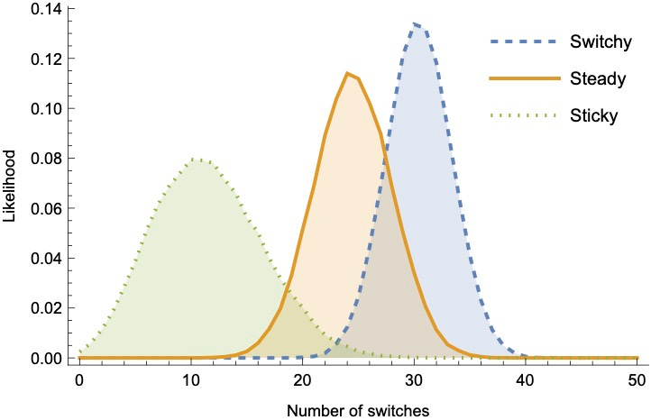
This means the likelihood distribution over data generated by Steady is closer to the distribution generated by Switchy than to the distribution generated by Sticky.³ We can visualize this looking at summary statistics of the sequences they generate—for example, the number of switches (Prius-to-Jeep or Jeep-to-Prius), the average streak-length, or the total number of Priuses. Here they are for sequences of 50 tosses—notice that in each case there’s substantially more overlap between the Steady and Switchy likelihoods than between the Steady and Sticky likelihoods.⁴

So Switchy generates data that is more-similar to Steady than Sticky does.

Why does that matter? Because it means that rational Bayesians observing unbiased data from the true (Steady) distribution will, on average, become doubtful of Sticky far more quickly than they become doubtful of Switchy.

To see this, let’s take a group of Bayesians who start out uniformly unsure between Switchy/Steady/Sticky, and then each observe a (different) sequence of n tosses, for various n. Here are their average posterior probabilities in each hypothesis, after observing the sequence:

Second Upshot: their average confidence in Sticky drops more quickly than their average confidence in Switchy.⁵ ‘

In other words: although our Bayesians converge to the truth (i.e. Steady), they do so in an asymmetric way—becoming more confident of Switchy than of Sticky along the way.

Now recall our First Upshot: whenever Bayesians are more confident of Switchy than Sticky, they’ll commit the gambler’s fallacy. Combined with the Second Upshot—that they on average will be more confident of Switchy than Sticky—it follows that, on average, Bayesians will commit the gambler’s fallacy.

Empirical Predictions

Okay. But do they do so in a realistic way?

Yes. I’ll focus on two well-known empirical effects. (The full paper addresses five.)

Nonlinear Expectations

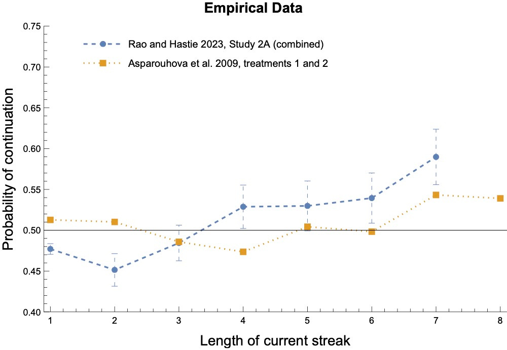
One of the most interesting empirical findings is that as a streak grows in length, people first increasingly exhibit the gambler’s fallacy—expecting the sequence to switch—but then, once the streak grows long enough, they stop expecting a switch and begin (increasingly) expecting the sequence to continue.

For example, here’s a plot showing the nonlinearity finding from two recent studies:

Our Bayesians exhibit nonlinearity as well.

Suppose we first let them update their opinions on Switchy/Steady/Sticky using either limited data (conditioning on a sequence of 50 outcomes, as above), or a simple model of limited memory (see section 4 of the paper for details). Then we show them a new streak and ask them how likely it is to continue.

What happens? They’ll first increasingly expect switches, but then increasingly expect continuations:

Why? Due to asymmetric convergence, they start out (on average) more confident of Switchy than Sticky. Because of this, as the streak grows initially, they think the process is increasingly primed to switch. That’s why they exhibit the gambler’s fallacy initially.

But as the streak continues, the streak itself provides more and more evidence for Sticky—after all, Sticky makes a long streak (which they’ve now seen) more likely than Switchy does. If the streak gets long enough, this provides enough data to swamp their initial preference for Switchy, so they start (increasingly) predicting continuations.

Experience-Dependence

A second finding is that the shape of these nonlinear expectations is experience-dependent. More precisely, two trends:

1. When people have more experience with (Steady) processes, they tend to deviate less from the true (50%) hit rate in their expectations.

2. For processes that they have little experience with, they transition rapidly from expecting switches to expecting continuations; but for ones they have more experience with, it requires a longer streak before they start expecting continuations.

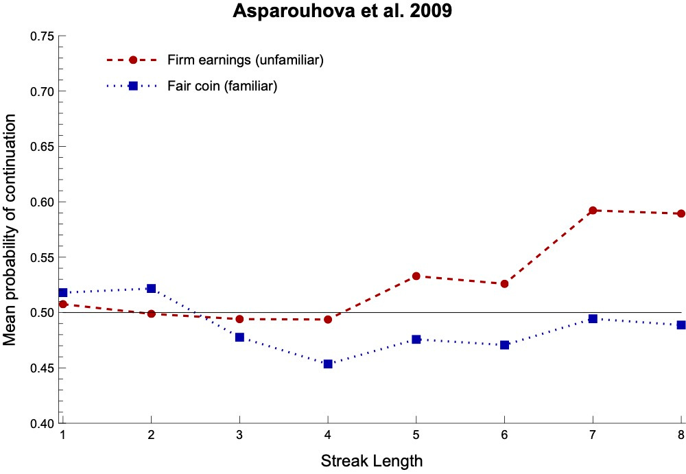
For example, here are the results for our above two studies when we separate out their experimental conditions by whether the process is familiar (blue)—such as a coin or urn—or unfamiliar (red/purple), such as a firm’s earnings or a stock market.

Notice that (1) their expectations for familiar processes stay closer to 50%, and (2) they take longer before that start expecting continuations (if they ever do).

Our Bayesians exhibit the same patterns. We can simulate this by varying how much data they’ve seen. When they have more data from a processes, they (1) stay closer to 50% in their expectations, and (2) take longer before they begin expecting continuations:

The results are qualitatively similar but more realistic if we consider agents with very (red) or somewhat (blue) limited memory:

Why? If they’re more familiar with a process, they (1) stay closer to 50% because they’re converging toward the truth: as they see more data, they get more confident of Steady, which pulls their expectations toward 50%. And (2) they take longer to begin expecting continuations because as they see more data, their opinions are more resilient: if they’ve seen a lot of data which makes them doubtful of Sticky, it takes a longer streak before the streak itself provides enough data to change this belief.

Other results

The paper considers three other results. Like real people, our Bayesians (i) produce “random” sequences that switch too often, (ii) change what they predict based on how often the sequence leading up to the prediction switched, and (iii) exhibit a form of format-dependence—appearing to exhibit stronger gambler’s-fallacy-effects when asked for binary predictions than when asked for probability estimates.

Moreover, the paper also shows that these results are robust to variations in the setup. The same qualitative results emerge even if our Bayesians are unsure about:

1. …the long-run hit rate (maybe it’s not 50%);

2. …how much the Switchy/Steady hypotheses deviate from 50% in their likelihoods;

3. …how these deviations build up as a streak grows;

4. …how exactly the Switchy/Sticky process shift probabilities over time.

So What?

Upshot: resource-limited Bayesians who are unsure of the causal structure of a process would exhibit many of the empirical trends that constitute our evidence that humans commit the gambler’s fallacy.

What to make of this?

You might think it’s all academic. For although real people exhibit the gambler’s fallacy for causal processes that they are reasonably uncertain about—parking battles, etc.—they also exhibit the gambler’s fallacy for coin tosses. And, you might think, people (should) know that coin tosses are Steady—coins have no memory, after all. So whatever they’re doing must be fallacious. Right?

Not so fast. To know that coin tosses are Steady just is to know that the next toss has a 50% chance of landing heads, regardless of how the previous tosses have gone. People who commit the gambler’s fallacy either don’t have this knowledge, or they don’t bring it to bear on the problem of predicting coin tosses. That requires some sort of explanation.

Here’s a cautious conclusion from our results: perhaps the above Bayesian process explains why. Most random processes—the weather, your mood, the stock market, etc.—are not as causally transparent as a coin. Thus people are (understandably!) in the habit of starting out uncertain, and letting the outcomes of the process shift their beliefs about the underlying causal structure. As we’ve seen, this will lead them to (on average) commit the gambler’s fallacy.

But more radical conclusion is also possible: maybe the gambler’s fallacy is not a fallacy after all.

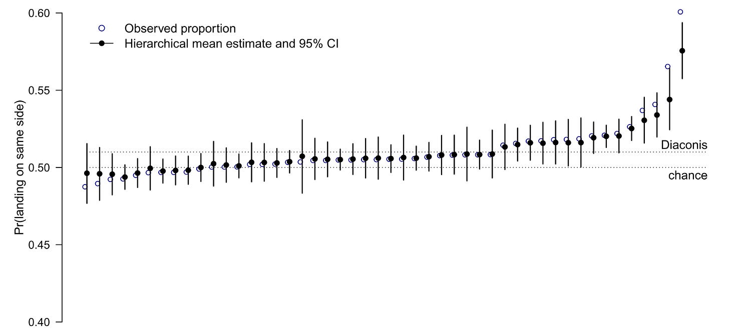
For coins are not as causally transparent as you think. In fact, it turns out that the outcomes of real coin tosses are not independent. Instead, they exhibit dynamical bias: since they precess (rotate like a pizza) as well as flip end over end, they are slightly more likely to land the way that was originally facing up when they were flipped. Classic estimates put this bias at around 51%.

Moreover, a recent study of 350,000 coin tosses found quite a lot of hetereogeneity in how much bias is exhibited. The average is around 51%, but individual flippers can vary quite a bite—many exhibit a dynamical bias of close to 55%:

And note: if our flipper turns the coin over between tosses, dynamical bias makes the outcomes Switchy; if he doesn’t, it makes them Sticky.

Upshot: coins are often either Sticky or Switchy.

Given subtle facts like this, maybe it’s rational for people to have causal uncertainty about most random processes—even coin flips. If so, they have to learn from experience about what to expect next. And as we’ve seen: if they do, it’ll be rational to commit the gambler’s fallacy.

So maybe the gambler’s fallacy doesn’t reveal statistical incompetence at all. After all, it’s exactly what we’d expect from a rational sensitivity to both causal uncertainty and subtle statistical cues.

---

What next?

• If you’re curious for more details, check out the full paper.

• For a recent, careful empirical study on the gambler’s fallacy, check out this paper.

• For other potential explanations of the gambler’s fallacy, see Rabin 2002, Rabin and Vayanos 2010, and Hahn and Warren 2009.

1. See Miller and Sanjuro 2018, which shows that the original studies purporting to show that the hot hand was a myth failed to control for a subtle selection effect—and that controlling for it in the original data reverses the conclusions. The hot hand is real.

2. By total probability and the Principal Principle.

3. Precisely: the KL divergence from Steady to Switchy is smaller than that from Steady to Sticky.

4. All graphs are generated using chains that linearly build up to a 90% switching/sticking rate after a streak of 5. Formally, the Markov chains for Switchy and Sticky are:

See the full paper for details. Section 6 of the paper shows that the results are robust to variations in the structure of the Markov chains.

5. Although in these plots you become doubtful of Switchy relatively quickly—after around 100 tosses—the paper shows that we get the same effect with arbitrarily-large amounts of data so long as our Bayesians have limited memory.