Bayesians Commit the Gambler's Fallacy

So real people might not be irrational for doing so, too.

[This post is based on a recently-published paper]

---

Baylee is bored. The fluorescent lights hum. The spreadsheets blur. She needs air.

As she steps outside, she sees the Prius nestled happily in the front spot. Three days in a row now. The Jeep will probably get it tomorrow—she’ll place her bet when she gets back.

Baylee’s not alone. Each afternoon in Bay City, her fellow office-mates check who won the morning’s battle for the front spot. It’s always either a Prius or a Jeep, and each manages to get it about half the time. But they all wonder about the fluctuations: if the Prius won the last few days, what are the chances it’ll win tomorrow? They place their bets with Bob.

In fact, the outcomes are statistically independent: each day, the Prius and Jeep each have a 50% chance of getting the front spot. But Baylee and company seem to think otherwise: when the Prius (or Jeep) is on a winning streak, she expects a switch is “due”.

Real people behave like Baylee: after a series of heads from a fair coin, they start to expect a tails. This is called the “gambler’s fallacy”—expecting random processes to be more inclined to “switch” than they actually are.

Does this imply that Baylee and company are irrational?

No. Baylee is a rational Bayesian. And real people who commit the gambler’s “fallacy” might be doing so for rational reasons.

How a Bayesian makes predictions

A “Bayesian” is an agent that assigns subjective probabilities to hypotheses, updates those probabilities proportionally to how well they explain the data, and makes predictions by averaging over the hypotheses.

For instance, suppose Baylee is unsure what is in a bag. She knows it contains 100 red and blue marbles, but is unsure of the proportion. She thinks it might include 25, 50, or 75 (of 100) red marbles. Imagine that she assigns 25% probability to the first hypothesis, 50% to the second, and 25% to the third:

• P( 25-red ) = 25%

• P( 50-red ) = 50%

• P( 75-red ) = 25%

Now what happens when she sees a red marble drawn from the bag, updating her probabilities to P⁺? She shifts probability from the first to the third hypothesis, since 75-red makes a red draw more likely than average:

• P⁺( 25-red ) = 12.5%

• P⁺( 50-red ) = 50%

• P⁺( 75-red ) = 37.5%

Notice two things. First, she doesn’t believe that the urn is mostly red—the most likely hypothesis is still that it has 50 red marbles.

But second, if we ask her to predict the next draw, she’ll predict red. For notice that the probabilities asymmetrically favor 75-red over 25-red. So when she averages the three hypotheses, weighting them by their probabilities, she’ll skew toward red:

\(P^+(\textit{next draw red}) ~=~ 0.125(25\%) + 0.50(50\%) + 0.375(75\%) ~=~ \textbf{56%}\)

The same process can explain the gambler’s fallacy.

Baylee knows that in the long run the Prius and Jeep each win the front spot half the time, but she wonders about the fluctuations. She considers three hypotheses:

1. Switchy: After a streak, a switch is more likely. (It’s like drawing from a deck of cards without replacement—after a few black cards, a red becomes more likely.)

2. Steady: Each time, the Prius has a 50% chance to win. (It’s like flipping a fair coin.)

3. Sticky: After a streak, a switch is less likely than a continuation. (It’s like having a ‘hot hand’.)

Suppose, again, she initially assigns the hypotheses 25%, 50%, and 25% probabilities:

• P( Switchy ) = 25%

• P( Steady ) = 50%

• P( Sticky ) = 25%

What will happen when she observes data?

Suppose she sees a random-looking sequence of Prius-wins (P) and Jeep-wins (J), such as PPPPJPJPJJ. This sequence has 4 ‘continuations’ of streaks (P to P, or J to J) and 5 ‘switches’ of streaks (P to J, or J to P). As a result, it’s more likely under Switchy than Sticky, so simulations show that her average posterior probabilities are:

• P⁺( Switchy ) = 20.2%

• P⁺( Steady ) = 70.4%

• P⁺( Sticky) = 9.3%

Again, notice two things. First, she doesn’t believe it’s Switchy—the most likely hypothesis is that it’s Steady.

But second, if we ask her to predict the next outcome, she’ll predict a switch. For her probabilities asymmetrically favor Switchy over Sticky. So when she averages the three hypotheses, weighting them by their probabilities, she’ll skew toward a switch¹:

\(P^+(\textit{switch}) ~=~ 0.202(70\%) + 0.704(50\%) + 0.093(30\%) ~=~ \textbf{52%}\)

She thinks it’s more likely than not to switch—she exhibits the gambler’s fallacy!

That’s no coincidence. Despite the apparent symmetry between Switchy and Sticky, it turns out that—if Steady is true—then it is easier to rule out Sticky than to rule out Switchy. Thus, as Bayesians observe data from an (in fact) Steady process, they will quickly rule out Sticky and slowly rule out Switchy, as in the above example. This asymmetric convergence toward the truth will lead them to, on average, commit the gambler’s fallacy.

Why is it easier to rule out Sticky than Switchy? The data generated by Steady turns out to be more similar to the data generated by Switchy than by Sticky. We can see this, for instance, by plotting the likelihoods of summary statistics—like number of Priuses (“hits”, left), or number of switches (right)—when we generate length-50 sequences:

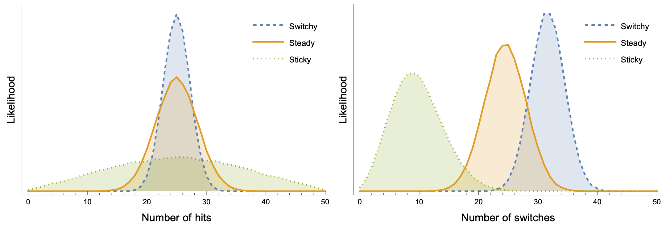
There’s more overlap between Steady (orange) and Switchy (blue) than Steady and Sticky (green).

As a result, if we generate random sequences and show them to Bayesians like Baylee, two things happen: (1) they converge to the truth, increasing probability in Steady; but (2) they do so asymmetrically—their probabilities for Switchy decrease slower than for Sticky.

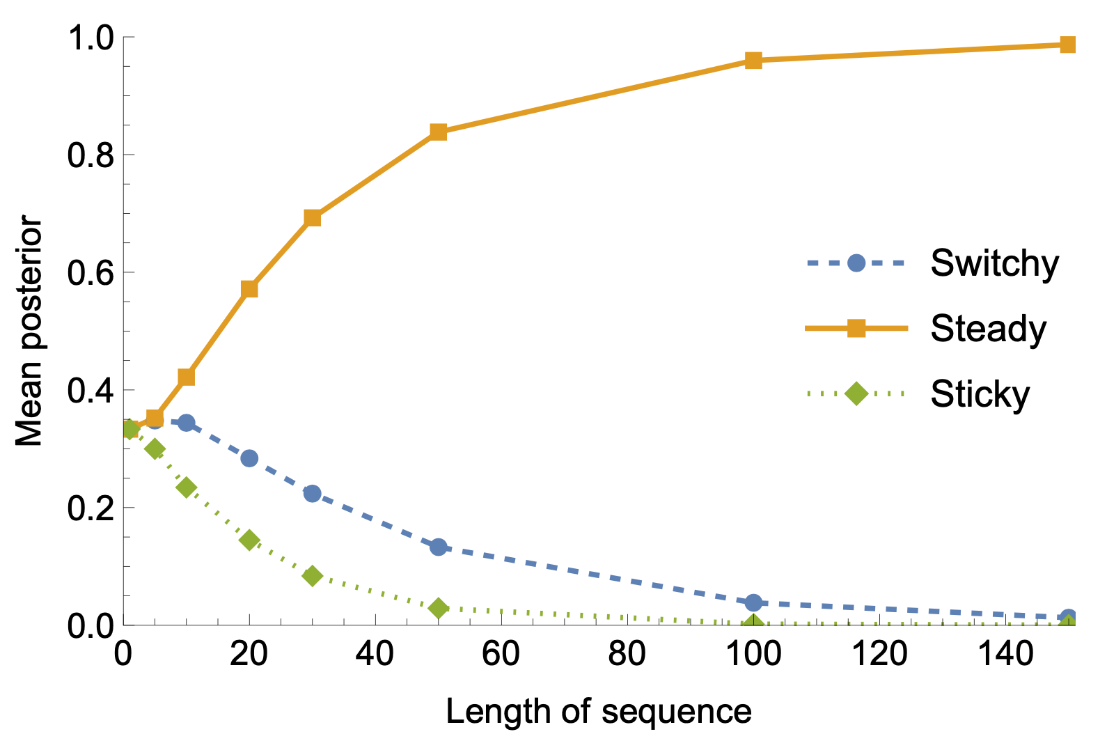
For instance, after seeing sequences of length 50, they on average (1) assign 83% probability to Steady; but (2) most of the remaining probability (14%) goes to Switchy, and only a little bit (3%) to Sticky. As a result, their average probability of a switch is 51.4%—on average, they commit the gambler’s fallacy.

This model also explains other empirical findings.

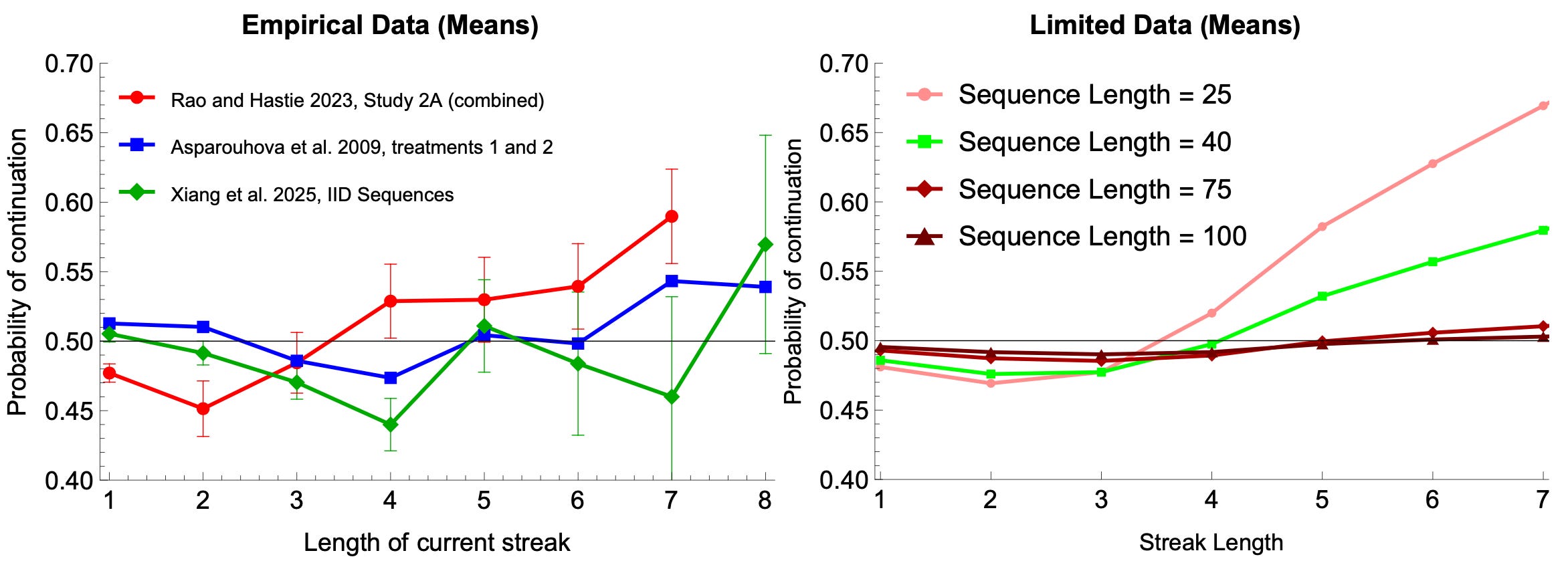
For instance, real people exhibit nonlinear expectations—expecting switches after short streaks but continuations after long streaks (below, left).

So do Bayesians: short streaks are evidence that the process is primed to switch, but long streaks are evidence that the process is Sticky—eventually leading them to predict continuations (below, right).

In short: the gambler’s fallacy might not be a fallacy at all—it might be explained by rational responses to causal uncertainty.

---

Curious about the details? Here’s the full paper.

1. Here assuming that after a streak of 2 jeeps (what she saw ended “…JJ”), Switchy makes a switch 70% likely, Steady makes it 50%, and Sticky makes it 30%.