A Subtle Selection Effect in Overconfidence Studies
Asking for confidence-intervals selects for the opinions that are most likely to be overestimated.
TLDR: The standard methods for studying overconfidence might be overestimating it. In asking people for confidence intervals—the narrowest intervals that they’re confident contain the true value—we’re selecting for the intervals that are most likely to be overestimates.
Fitz the fisherman assures you that all the fish in this cove are big—he’s been fishing in these waters for decades, and he’s never caught one smaller than 6 inches. You’re skeptical. What’s the first question you should ask?
“How big are the holes in your net?”
This is a classic example of a selection effect: if Fitz’s net has holes bigger than 6 inches, then he’d never catch small fish even if the cove is full of them.
Selection effects are a thorn in the side of calibration research: the subfield of psychology that tries to test when and why people are overconfident in their beliefs.
There are various approaches, but the method known as “interval estimation” asks people for intervals that they are confident contain the true value of some unknown quantity.
For example, “What proportion of Republicans think that racism still exists in America?” Take a second and make an interval that you’re 90%-confident contains the true proportion. Then check the answer in the footnote.1
Most people are overprecise: their intervals contain the true value far less than 90% of the time. Overprecision has been called the “mother of all biases” due to both its robustness and importance.
The previous post argued that many of the surprising findings surrounding overprecision make more sense once we realize that subjects aim to give answers that are informative relative to the question under discussion.
Today, I’d like to propose a complementary hypothesis: overprecision studies suffer from a subtle selection effect that (to my knowledge) has not been corrected for.
The History
First some history. Calibration research began in earnest in the 70s, when psychologists started to put the presuppositions of economic models to the test. Were people as rational and well-calibrated in their opinions as standard models of the free market assumed?
The original way to test for overconfidence was to ask people trivia questions, have them rate their confidence in their answers, and then record what proportion of answers were true at each level of confidence. If people are perfectly calibrated, this will form a diagonal line: of all the claims people are 50%-confident in, 50% will be true; of all the ones they’re 60%-confident in, 60% will be true, and so on.
At first, the overconfidence effect was thought to be standard: on average people were much more confident in their opinions than was borne out in their accuracy. For example, of all the opinions they are 80%-confident in, only 60% were true. This can be seen in the following graph from this widely-cited early study—note that the “proportion correct” (y-axis) amongst all the judgments they’re 80%-confident in (x-axis) is only around 60%:
But there was a problem. It was soon realized that the overconfidence effect wasn’t robust, and instead was an illusion driven by a selection effect. In trying to find questions that subjects’ were uncertain about, researchers were accidentally selecting questions that were hard to get right. This is intuitive when you think about it: no one asks easy questions like “ What’s the capital of the US?” in a trivia exam!
The result was that the overall proportion of true guesses (“hit rate”) on these tests was much lower than it would normally be. If hard questions are big fish and easy questions are small fish, researchers were—like Fitz—fishing with a big net: they were missing all the easy questions in which people tend to underestimate their accuracy.
It’s now widely appreciated that to avoid this, calibration tests must be constructed randomly from a natural domain—for example, comparing pairs of random cities and guessing which one is larger. Once this is done, it was found that subjects exhibit the hard-easy effect: on exams where it’s hard to guess correctly, people overestimate their accuracy—but on exams where it’s easy to guess correctly, people underestimate their accuracy.
The hard-easy effect is extremely weak evidence for overconfidence—even ideally rational Bayesians would exhibit it. After all, even rational people will be confident of some claims that are false and doubtful of some claims that are true. By definition, hard tests select for the former, while easy tests select for the latter.
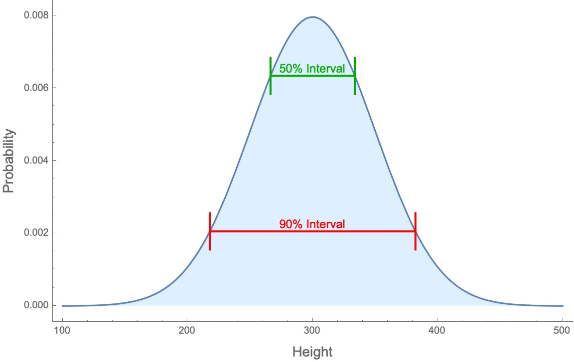
This is one of many reasons why a different type of calibration test is now taken to be the strongest evidence for overconfidence—namely interval estimation. As discussed in the previous post, this method asks for estimates of an unknown quantity, like “How tall is Niagara Falls?” Your 90%-confidence interval is the narrowest interval that you’re 90%-sure contains the true value. So if your uncertainty about the possible values is represented by the bell curve below (with height corresponding to how likely they think that value is), your 90%-confidence interval is the red interval right in the middle:
Those 90%-confidence intervals are calibrated if 90% of them contain the true value; they are overprecise if less than 90% of them do.
The main empirical finding of the interval-estimation literature is that people are almost always overprecise, and almost never underprecise. This contrasts sharply with the “hard-easy effect”—which, recall, found that people underestimate their accuracy on easy tests.
As a result, many researchers have concluded that the robustness of overprecision provides the best evidence for overconfidence.
A Hidden Selection Effect
But here’s a puzzle. We can simulate Bayesian agents who have uncertainty about a quantity—say, the average height of skyscrapers in Boston.2 Now we’ll ask these agents two types of questions:
Ask for their 90%-confidence intervals for that average height.
Provide them with a randomly chosen interval, ask them how confident they are it contains the true average value, and then throw out intervals that they’re not exactly 90%-confident in.
For example, in the below picture the red interval is their 90%-confidence interval, the other colors are random intervals. We would throw out the green, orange, and blue intervals (since they’re not 90%-confident in those), but keep the purple one in the data set (since they’re also exactly 90%-confident in it).
How do you think the hit rates of (1) and (2) will compare? Both will consist of intervals that they are exactly 90%-confident in—the former given directly, the latter selected randomly.
Intuitively, they should be the same. I certainly thought they would be.
But that’s wrong. For example, consider agents who start out overprecise, and then compare the hit rates of the two types of intervals as they observe an increasing number of datapoints (i.e. are told the heights of various random skyscraper in Boston). Here’s a plot of their hit rates—the proportions of each type of interval that contains the true value:
Both types of intervals are overprecise—they have hit rates below 90%. But the 90%-confidence intervals are significantly more overprecise than the random intervals, and they only slow converge toward calibration with increasing data.
The same dynamic holds if we start with agents whose priors are underprecise:
Or whose priors on random intervals are calibrated:
In each case, when we elicit confidence intervals, our (Bayesian!) agents look more overprecise than when we ask them about their confidence in random intervals. And this is happening despite the fact that these are two ways of asking about the same underlying probability distributions of these agents.
What’s going on?
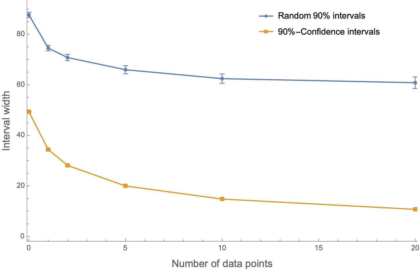
The trick is to remember how confidence intervals are defined: your 90%-confidence interval is the narrowest interval that you’re 90%-confident contains the true value. In other words, any other random interval that you’re 90%-confident in will be wider. Notice, for instance, that the purple random interval in the diagram above is significantly wider than the red interval.
We can verify this by running the same simulations and then tracking the average width of intervals. (If the interval is “between 150–255”, the width is 105.) The result? The random 90%-intervals are way wider than the 90%-confidence intervals:
That means we’ve run into another selection effect.
Now, we know that if their overall probabilities are not well-calibrated, then in general their intervals won’t contain the true value exactly as often as they expect—they’ll be overprecise or underprecise.
But when we ask for the narrowest interval they’re 90%-confident in, we are implicitly selecting for the interval they’re the most overprecise on, since by definition narrower intervals have less of a chance of containing the true value than wider ones.
Like Fitz the fisherman—who missed all the small fish because his net had big holes—in asking for 90%-confidence intervals we’re going to miss all the wide intervals that people are 90%-confident in, which are the ones that are most likely to be underprecise.
So what?
What to make of all this? There are obviously many factors that contribute to overprecision, and this doesn’t explain them all. But I think it’s fair to say that the main interest in interval elicitation is due to the fact that it purportedly leads to much more extreme and robust evidence for overconfidence than other measures.
What we’ve found is that we should expect more overprecision from interval elicitation than from those other measures: interval elicitation selects for the intervals which are most likely to regularly miss the true value.
Although researchers in this area are generally sensitive to selection effects, I’m not aware of any cases where they have explicitly acknowledged and controlled for this one. Have they?
If not, how much does this selection effect dampen the claim that overprecision provides the best evidence for overconfidence?
To avoid being overprecise myself, I’ll hedge and say: at least a little bit.
What next?
If you know of cases of researchers controlling for or measuring this selection effect, please let me know!
For another hypothesis about why the evidence for overprecision may be overstated, see the previous blog post.
In these simulations, the quantity was the mean of a normal distribution with known variance; agents started with random (normal) priors that varied across simulations in how close their means were to the true distribution, and hence how over- or under-precise the agents’ priors were. Agents then observed data generated from the true distribution and updated in a Bayesian way.


